GPU PDE Lab
In service Sep 2026Finite-difference PDE solvers written from scratch, an interactive lab to drive them, and a measurement of how much of a GPU they actually use. The obvious way to write a 5-point stencil in PyTorch reaches 7% of this card’s achievable memory bandwidth. A hand-written fused Triton kernel computing the identical update reaches 93%.
93% of achievable bandwidth, fused Triton kernel
7% of achievable bandwidth, eager PyTorch
4.2–12.9× faster, measured on an RTX 2080 Ti
Where the idea came from
This started from misreading a course title. ETH Zurich runs a course on solving PDEs in parallel on GPUs, and I assumed going in that it was about clever parallelization tricks for approximating solutions to particular equations. It is closer to the opposite: you numerically push the starting state of a field forward in time under whatever PDE governs it, which means touching every cell on every step. Once I understood that, the parallelism angle became obvious, since the field itself is the natural unit of work, and that was the premise of the app.
What I built first was that app: twelve interactive experiments across heat, wave, Poisson and 2D fluid, every stencil and time-stepper and iterative solver written from scratch in plain array operations. PyTorch is an execution engine in it, not a PDE library. That part worked, and I was reasonably happy with it, and it was also where I stopped thinking.
The question I had not asked
The app could tell you the GPU was faster than the CPU. It could not tell you whether the GPU was being used well, and I had quietly assumed those were the same question. They are not. A 5-point stencil does about six floating-point operations per eight bytes it moves, which puts it far below the point where arithmetic throughput matters at all. The only thing that determines its speed is memory bandwidth, so the real question is what fraction of the available bandwidth you are getting.
I measured it. The answer was 7%.
The cause is not exotic. Writing the update as shifted-slice arithmetic, which is the readable, idiomatic way, makes every intermediate expression its own full-sized array with its own round trip to memory. Counted at PyTorch’s dispatch layer, one heat step makes about 33 passes over memory where one read and one write would do, spread across 17 separate kernel launches. My own documentation had estimated four passes. It was off by a factor of eight, and I only found that out because I stopped estimating and measured.
Four ways to take one step
So I wrote the same heat-equation step four times and timed them against each other, with every version checked for agreement against the original at every boundary condition and both precisions.
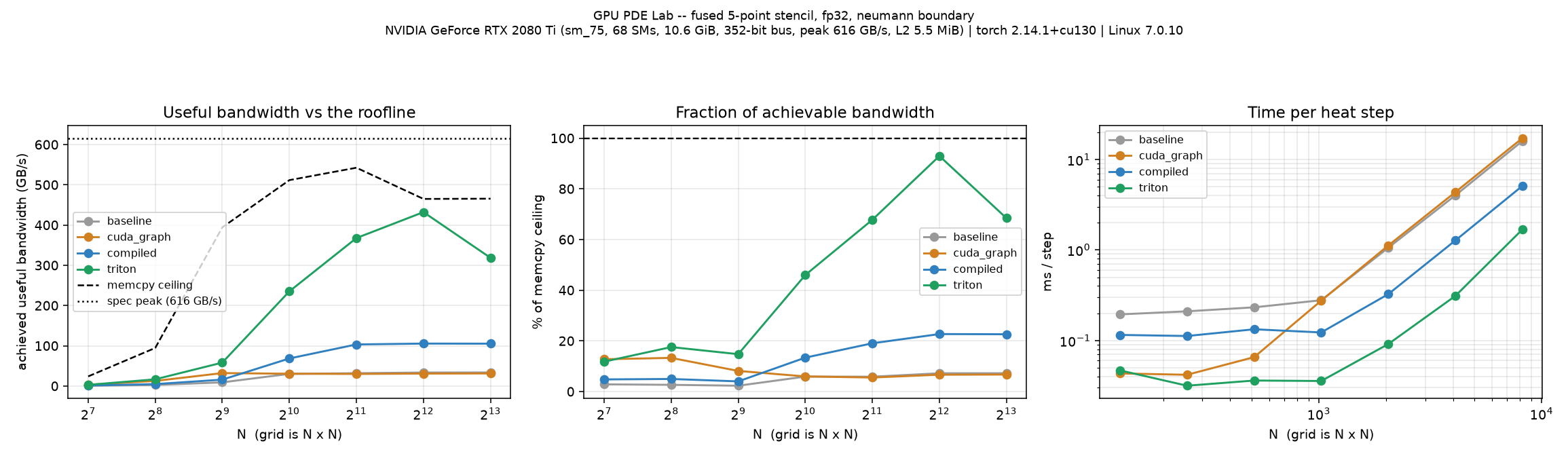
python scripts/run_roofline.py; raw numbers are committed alongside the figure.The hand-written Triton kernel is the one that matters: a single fused kernel, one read of the field, arithmetic in registers, one write. It runs 4.2 to 12.9 times faster than the original depending on grid size, and reaches 93% of what a plain memory copy achieves on the same card, which is about as close to the floor as a stencil can get, since a stencil cannot beat a memcpy.
The fiddly part was folding the boundary condition into the same pass instead of paying for a second kernel launch. A boundary cell’s value depends on an interior cell that a different thread block computes, and there is no ordering between blocks inside one launch. The way out is to recompute rather than read: every cell evaluates the stencil at its own index clamped into the interior. An interior cell clamps to itself and is unaffected; an edge cell lands on its inward neighbour, which is exactly the value the boundary condition says it takes; a corner clamps on both axes and lands on its diagonal neighbour, which is what the original’s four sequential edge writes leave behind. The redundant work is a few hundred cells out of millions.
The result I kept because it is negative
One of the four implementations captures the original operations into a CUDA graph and replays them as a single submission. It removes the cost of launching seventeen kernels and changes nothing about the memory traffic.
It wins 5× on a 128×128 grid. On anything from 1024×1024 upward it loses: 0.92×, slightly slower than doing nothing.
That is the most useful thing in the whole comparison and I nearly dropped it for looking like a failure. “The GPU is slow” is two completely different problems with two unrelated fixes: on small grids you are paying launch overhead and the graph is the answer, on large grids you are paying for memory traffic and only fusion helps. A single wall-clock number cannot tell you which one you have. Running both, including the one that regresses, can.
In the same spirit: torch.compile gets you from seventeen kernels to four with no new code, and reaches 23% of the ceiling. It fuses the arithmetic but not the in-place boundary writes, which is precisely the gap the hand-written kernel closes. Three and a bit times better than free is a real result, and it is also the number that makes the Triton figure mean something: beating eager proves nothing about a kernel, beating the compiler does.
Two bugs worth recording
Triton binds a Python float kernel argument as fp32. Passing the grid spacings and the timestep coefficient as plain scalars silently truncated them, so an fp64 field was being stepped with single-precision coefficients and carried about 1e‑8 relative error. Nothing crashed and nothing looked wrong; it would have quietly corrupted the fp16/fp32/fp64 precision comparison the project exists to make. I found it because one grid size showed an error seven orders of magnitude above machine epsilon and I did not want to round it off as noise. The coefficients now travel in a tensor of the field’s own dtype, and a test holds them there.
The second is smaller and more embarrassing: the Jacobi iteration allocated its output with field * 0.0, reading an entire array in order to multiply it away. My own stencil module has a comment explaining why that is wrong. I had written the comment and then made the mistake again in the other hot path, the one that runs dozens of times per frame in both the Poisson solver and the fluid pressure projection.
Where it stands
162 tests. Every optimized kernel is checked against the original at every boundary condition, both precisions, and deliberately ragged non-power-of-two grids where tile masking is most likely to go wrong; the eager reference is asserted bit-identical to the solver it stands in for, so it cannot drift from what it represents. CI on two Python versions, lint and type checking clean over the solver and measurement layers. Figures are generated by running the solvers rather than screenshotted, so one that stops matching the code shows up as a diff.
The container image is built and exercised, not just written: the suite runs inside it unaided, 131 passed and 31 skipped, the skips being the CUDA tests correctly declining a GPU-less container. Two things fell out of that worth more than the image itself. The kernel counter reports the same 33 array passes from inside Ubuntu that it reports on my NixOS host, and regenerating the figures in the container produces files that are bit-identical by checksum to the committed ones. The claim that these figures are generated rather than screenshotted is therefore demonstrated across two unrelated toolchains rather than asserted.
What is not done: 3D covers the heat equation only: wave, Poisson and fluid would each need their own numerical work rather than a reuse of the existing solver. The pressure solves run on a fixed iteration budget for interactivity instead of solving to convergence, with the residual plotted so the approximation is visible rather than hidden. The pass counts are requested traffic measured at the dispatch layer, not DRAM transactions, so they are an upper bound that is only tight once the field no longer fits in cache.
MIT-licensed, and there is a Colab notebook if you want to run the convergence study and the roofline sweep on a free T4 without installing anything.